class 05

Author

Chen

Background

There are lots of ways to make plots in R. These include so-called “base R” (like the plot()) and on packages like ggplot2.

Let’s make the sampe plot with these two graphics systems. We can use the inbuilt cars dataset:

shortcut: option+command+i(insert)

head(cars)

  speed dist
1     4    2
2     4   10
3     7    4
4     7   22
5     8   16
6     9   10

With “base R” we can simply

plot(cars)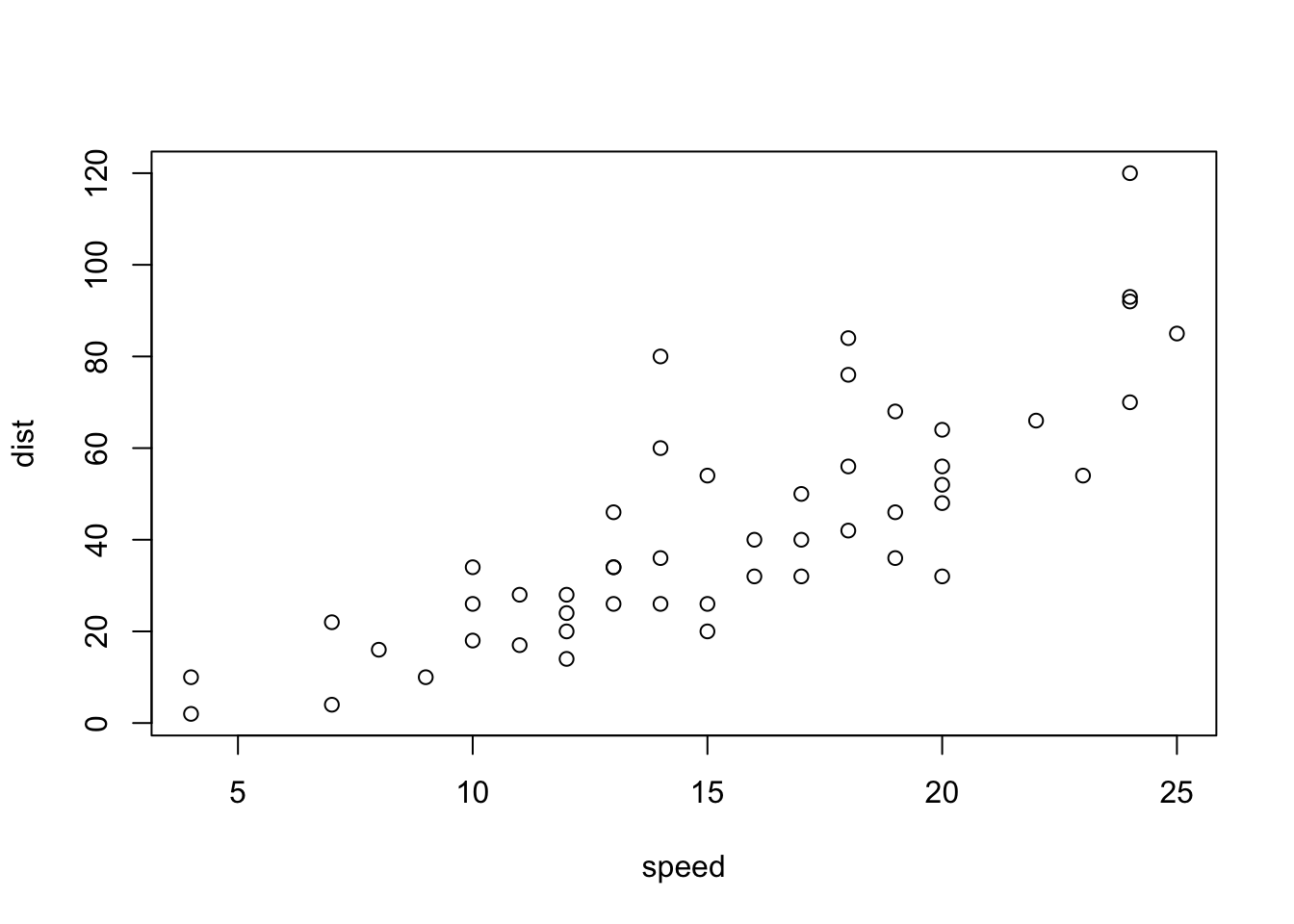

Now let’s try ggplot. First I need to install the package using install.packages("ggplot2").

N.B. We never run an install.packages() in a code chunl otherwise we will reinstall needlessly every time we render the document.

#———-not use for now————-

url <- "https://bioboot.github.io/bimm143_S20/class-material/up_down_expression.txt"
genes <- read.delim(url)
head(genes)

        Gene Condition1 Condition2      State
1      A4GNT -3.6808610 -3.4401355 unchanging
2       AAAS  4.5479580  4.3864126 unchanging
3      AASDH  3.7190695  3.4787276 unchanging
4       AATF  5.0784720  5.0151916 unchanging
5       AATK  0.4711421  0.5598642 unchanging
6 AB015752.4 -3.6808610 -3.5921390 unchanging

nrow(genes)

[1] 5196

ncol(genes)

[1] 4

table(genes$State)


      down unchanging         up 
        72       4997        127

table(genes$State)/sum(table(genes$State))


      down unchanging         up 
0.01385681 0.96170131 0.02444188

1+1

[1] 2